A multi-layer AI decision support system for startup success prediction and risk assessment using knowledge graphs and federated learning – Scientific Reports

This section discusses the dataset used for this study and proposed a model for predicting the startups success or failure.

Data used

Our data sample was taken from Crunchbase’s August 2018 Daily CSV Export. The complete dataset includes 227,172 tuples describing fundraising round events (mostly from the last 20 years), information about 799,446 firm founders, and 623,232 companies²³.Given the significant failure rate in the early years, for instance, it was roughly 44% in the US at four years and these windows are deemed sufficient for a company²⁴. Research by Arroyo et al. served as the foundation for our data selection process. Initially, startups founded between March 2014 and March 2018 were taken into account. Startups that have advanced to the next level of the C series and have been purchased, closed, or listed on an initial public offering (IPO) during this time have not been included. because early-stage investments don’t appeal to them.

Significant changes in commercial ecosystems are captured during this time, providing a wealth of data for examining survival paths. The authors’ 10 years of working with startups, which gave them exclusive access to context-rich data from both successful and unsuccessful endeavors, influenced the data collection approach.All responses were gathered using structured questionnaires to reduce the possibility of subjective bias. Semi-structured interviews were added, and the results were cross-validated against publically accessible data to guarantee consistency and dependability. Startup managers were given structured questionnaires with 81 items that focused on essential survival traits. Semi-structured interviews with investors, entrepreneurs, and other stakeholders were added to these to provide more qualitative depth. While secondary data, such as financial records, fund-raising histories, and reports on the market ensured a comprehensive perspective, observations made during startup operations offered additional insights. This combination of data sources improves contextual relevance and reliability while adhering to standard practices in startup research. Finding the startups that have the potential to succeed and those who have already done so was the next stage. Investors’ ultimate goal is an IPO. Nevertheless, it is uncommon for businesses to reach the initial public offering (IPO) stage, with 30% of seed-funded businesses exiting through an IPO²⁵. Investors look for businesses that will advance toward new funding infusions and possibly better outcomes. Additionally, they seek for businesses that will invest rapidly in order to grow more swiftly on their own²³. For a more thorough assessment of potential investments, we therefore took into account both partially successful and acquired startups in addition to successful startups. Successful startups are those that made it to the initial public offering (IPO) stage between March 2018 and March 2021. Additionally, businesses who have raised additional capital throughout this time frame are regarded as partially successful start-ups.

The collected attributes are based on five dimensions such as team-dynamics, financial metrics, and conditions of market, service and product differentiation and the vision of strategic. Qualitative responses were transformed into statistical scores using a systematic coding methodology to guarantee the data’s quality and reproducibility. Throughout the procedure, logs were kept that detailed the nature and provenance of each feature. On a scale of 0.0 to 1.0, survival outcomes were represented, where 1.0 denoted completely successful companies that showed consistent growth and market presence. Firms that experienced difficulties with financial stability or market adaptation and had only partial success were given values below 1.0, whilst failing firms that completely stopped operations were given a rating of 0.0.

Model explanation

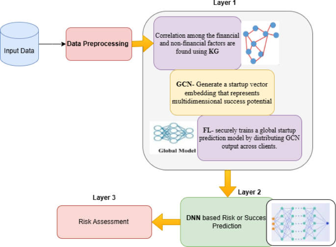
Figure 1 illustrates the model structure of the proposed multi layer decision support system for predicting the startup survival based on the risk and success. A multi-layer decision support system designed for risk assessment and startup success prediction. As shown in the Fig. 1, the proposed framework combines Federated Learning (FL), Graph Convolution Networks (GCN), and Knowledge Graphs (KG). The process begins with preprocessing the input data, which includes collecting and classifying startup-related financial and non-financial data. A KG is then constructed to identify correlations and semantic links among elements of financial and non-financial factors of startups. A GCN receives this improved representation and uses it to train multidimensional embeddings for each startup by aggregating data from its graph-based neighborhood. These embeddings indicate the startup’s overall success. To preserve data privacy and promote inter-institutional collaboration, a global predictive model is trained among scattered clients via FL.

Overview of proposed multi layer decision support system to predict startup survival.

Although we recognize that federated learning (FL) and graph convolutional networks (GCNs) have been used in other fields, our work is innovative in the way these techniques are modified, expanded, and contextualized for the startup forecasting challenge. Startups face particular difficulties, including a lack of organized datasets, confidentiality restrictions, and extremely varied data (finance indicators, team structures, market situations, and product features). Our approach goes beyond a straightforward GCN and FL combo to solve these issues by including a number of methodological improvements which is shown in Table 1. By adapting GCN and FL to the features of startup ecosystems, we are able to go beyond their conventional use cases and provide both methodological originality and usefulness. These improvements allow the model to produce actionable insights for practical decision-making in the entrepreneurial domain in addition to producing accurate predictions.

Layer 1: correlation among influencing factors and its extraction using KG-GCNFL

1. (i)

   Preprocessing to handling missing values

The quality of features embeddings in the Graph Convolutional Network (GCN) model may be impacted by the missing values we found in the history records of start-up businesses during our investigation. This study used two imputation methods such as mean imputation and K-Nearest Neighbors (KNN) imputation—to solve this problem. In mean imputation, the mean of the observed values for that feature is used to fill in the missing values. When the data are Missing Completely At Random (MCAR) and the percentage of missing data is low, this approach is simple and efficient. However, if the missing data are not MCAR, it may induce bias and decrease variability²⁶. In contrast, KNN imputation takes into account the similarity between data points and guesses missing values using the values of the ‘k’ nearest neighbors. Because it maintains the underlying data distribution and interactions among features²⁷, this approach is more reliable, particularly when the data are Missing At Random (MAR). We improved the GCN model’s performance and dependability by using these imputation techniques to make sure the feature embeddings input into the model were comprehensive and representational of the underlying data.

1. (ii)

   Startup Knowledge Graph (SKG)

Google was the first to propose the knowledge graph, which is essentially a semantic network that describes objective items and their interactions in the form of graphs, exposing the relationships between entities. The network’s edges are made up of the relationships between the entities, which can be expressed as (head entity, relationship, tail item) triplets. The entities that exist in the objective world are equivalent to the entities in the network.

Given a graph G={V, E}²⁸, where V denote collection of nodes, E denote the set of edges and it is extended for KG as,

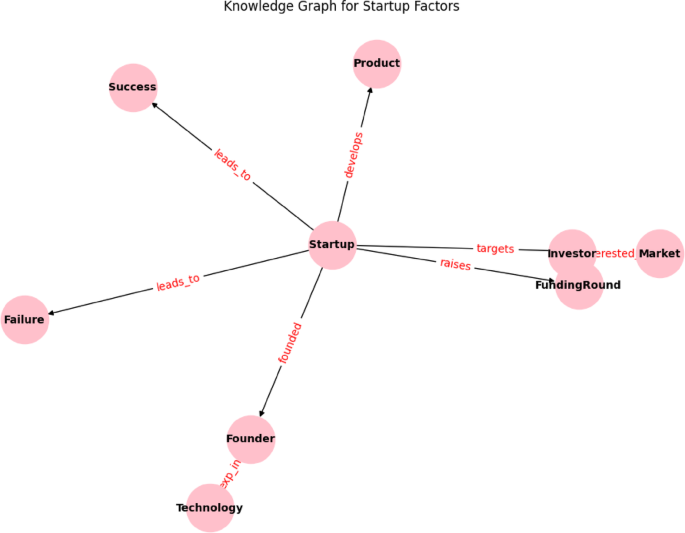
where V is the set of nodes \(V=({v}_{1},{v}_{2,}\dots{v}_{n})\) which is categorized into types called \(T=({t}_{1},{t}_{2,}\dots{t}_{t})\) such as founders, investors, markets, products, competitors and so on. \(E\subseteq(V,V)\) is the collection of edges \(e=({v}_{i},{v}_{j})\) denotes the relationship among the nodes \({v}_{i}\;and\;{v}_{j}\) which includes founders has an experience with industry, startup has funding from investor and founder worked at the successful company and so on. R denotes the types of relationship and describes its nature of interactions. \(\phi\)is a function which assigns the relationship type r to R of each edge e and \(\psi\) is a function assign a type T to each node v. Figure 2 illustrates the KG for the considered data. The entities of the graphs are {Startup, Investor, Founder, Product, Funding Round, Market, Technology, Failure, Success} and their relationships are denoted in edges which includes in Table 2. While manual intervention is mainly restricted to initial schema design and periodic validation, automated data ingestion pipelines that update entities and relationships from external startup databases and funding records can maintain the knowledge graph in operational settings. The knowledge graph format allows for the insertion of region-specific traits or entities to capture local ecosystem characteristics while maintaining the basic entities and linkages across various geographic startup ecosystems.

Knowledge graph of startup success and risk prediction using the proposed multi-layer decision support system (MLDSS).

1. (iii)

   GCN-FL

When it comes to handling spatial relationships between things, GCNs²⁹ have shown remarkable performance. In order to address the spatial relationships between nodes, they seek to combine the data of nodes and their neighboring nodes. Because of the influence of nearby and distant points, the closer the neighboring points are, the more of an impact they have and each node modifies its state until the ultimate equilibrium. The adjacency matrix contains this pertinent data. The GCN used here is for feature extraction. Suppose, we have the batch of graph that contains N nodes, and each nodes has its own features, that form the matrix \(X \in ^{{N*k}}\), where k is the index number. The nodes relationship forms the adjacency matrix \(A\in{R}^{N*N}\). The GCN aggregates the feature information to form the local neighborhood as,

where D is the degree matrix of A which is the adjacency matrix, \({H}^{l}\)is the intermediate hidden embeddings ateach layer l which is denoted as (H⁰ is X), W is the weight matrix of layer l. \(\sigma\) is the ReLU activation function. In this Z = H^(l) is the final node embeddings to represent the potential of startup success.

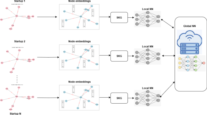
Figure 3 shows the GCN-FL framework that comprised of multiple SKG for decentralized learning without required the raw or private data. This model comprised of various SKG’s, each denotes the relationship of various factors of startups. To prevent direct sharing of data and considering the privacy and security, FL framework is incorporated to facilitate the global model training.

The devloped GCN-FL framework.

Let there are C companies, each with local data set D_c, and local processed embeddings using GCN called Z_c. Each startup trains it owns local model weight as W_c using the embeddings and labels to reduce the loss as:

where \(f{w}_{c}\) is the output of local prediction, Z is the embedding of feature i, Y is the output of predicted probability of two nodes and l is the loss function. In order to ensure that customers with more data contribute proportionately to the global model, we specifically use weighted aggregation based on the amount of local samples per client. To lessen distributional discrepancies prior to aggregation, we also apply feature scaling and local normalization to every client. We periodically evaluate local models and dynamically modify aggregation weights to further limit performance loss caused by non-IID data. The central server of FL aggregates the update from all the companies local NN using FedAvg:

where \({W}_{t}\) is the global model and \({n}_{c}=\left|{D}_{c}\right|\), \(n=\sum_{c}{n}_{c}\). This aggregated model is further redistributed to find the best output until convergence. The aggregated features of both financial and non financial factors are listed in Table 3.

We carried out a comparative analysis with a non-FL centralized configuration in order to confirm the efficacy of the FL framework. The Results section reports the specific performance differences in terms of accuracy, F1-score, training duration, and communication overhead.

Layer 2: prediction using DNN

The unified feature vector from the GCN-FL is fed as input to DNN for success or failure prediction since it serve as the major predictive factor of proposed DSS. Deep-level interactions among heterogeneous features are extracted by the DNN’s several nonlinear transformation layers. The last layer produces a binary classification result that shows whether a startup’s funding round is expected to be successful or unsuccessful. The DNN receives the output Z of the embeddings from GCN and outputs the probability as \(\hat{Y}\).

Let, \(Z\in{R}^{n*d}\) is the input matrix from GCN, w^l and b^l are the weight and bias of layer l and L is the number of layers in DNN. The prediction from DNN is expressed as,

Final output as success or risk is predicted as,

where OL is the output layer value. The framework uses optimization techniques such the Binary Cross-Entropy Loss as a goal function to further improve the forecast dependability of the system. This loss function ensures reliable model training for practical use in decision support scenarios by efficiently measuring the difference between expected probability and actual outcomes.

where \((1 – (\hat{Y}_{i} )\) is the probability of failure (risk score) among the value 0 and 1. This score denotes the startup success or failure of proposed model confidence. A high value of 1 denotes the success and low value 0 denotes the risk of failure. A grid search approach in conjunction with 5-fold cross-validation was used to refine the DNN model in order to guarantee optimal performance and reproducibility. The number of hidden layers (2–5), the number of neurons per layer (64–512), the optimizers (SGD, Adam), the activation functions (ReLU, tanh, sigmoid), and the learning rates (0.0001–0.01) were among the configurations that were examined. Three hidden layers with 256, 128 and 64 neurons each, followed by a ReLU activation and a dropout rate of 0.3 to avoid overfitting, made up the final design. With a learning rate of 0.001 and categorical cross-entropy as the loss function, the Adam optimizer was used to train the model.

Qualitative responses from semi-structured interviews and structured questionnaires were quantified using a predetermined coding methodology in order to methodically include non-financial aspects in the predictive model. Standardized criteria were used to categorize or assign numerical values to each response. For example, open-ended interview inputs were thematically examined and transformed into categories or numerical representations, while team experience, market involvement, and product distinction were categorized into ordinal or binary scales. For thorough startup success and risk prediction, non-financial attributes can be combined with financial measurements using this method, which guarantees consistency and repeatability throughout the dataset (see Table 4 for the coding scheme).

Risk assessment

The risk identification and assessment are the third layer of the proposed Multi layer DSS system. Within the startups, the risks are need to be identified which is stated in Table 3. The identified risk is analyzed level of risk severity is computation shown as follows:

where \(Severity\) is the impact of occurrence of risk (1-negligible, 10-catastropic), Occurrence denotes the likelihood of the occurrence of risk (1- rare, 10- frequently) and Detection is the ease of identifying the risk (1- very likely, 10-hard to detect).